The Phenomenon That Can Destroy a Pipeline in Milliseconds

Water hammer is one of the most dangerous overpressure phenomena in liquid pipeline systems — and one of the most misunderstood.

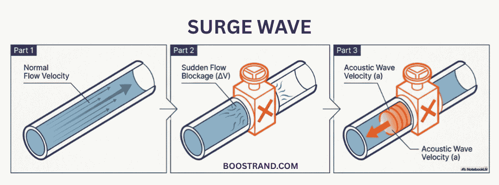
Picture a pump discharging into a long pipeline. At the far end of that pipeline, there is a receiving tank with a shutdown valve on the inlet. Now imagine that a shutdown valve closes suddenly at the end of the pipeline. The flowing liquid does not stop all at once — it cannot. The momentum of the entire liquid column is still pushing forward, and the sudden closure creates a shockwave that travels backward through the pipe, slamming into the still-incoming flow from the pump. This is water hammer.

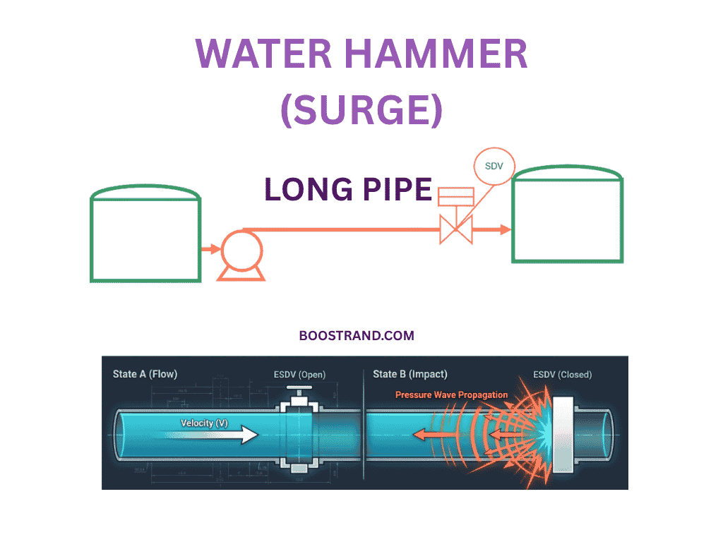
This phenomenon is particularly severe in long liquid pipelines for a specific reason: the greater the pipe length, the more time it takes for the pump to “sense” any downstream resistance. By the time the pump responds, the shockwave has already propagated back through the system, and the two pressure waves collide.

Three characteristics make water hammer uniquely dangerous compared to ordinary overpressure events:

• The pressure rise can far exceed pump shutoff pressure — even reaching multiples of the normal operating pressure
• The overpressure is localized — concentrated in specific pipe segments rather than distributed along the line, making certain points disproportionately vulnerable to failure
• It is instantaneous — conventional protection methods such as PSVs or shutdown systems do not have time to respond before the peak pressure is reached

This last point is critical. That’s why conventional Pressure Safety Valve (PSV) requires several seconds to sense the overpressure, open, and relieve. A surge pressure event can peak and begin to cause structural damage in under one second. This is precisely why water hammer must be studied using dedicated dynamic simulation software — not addressed as an afterthought with a standard process relief valve.

In this article, we shall go through the basic premises needed for surge analysis, common surge protection methods and basic design criteria for a surge relief system.

---

Maximum Allowable Pipeline Pressure for Surge Analysis

Before carrying out the surge analysis to determine the peak surge pressure, it is essential to understand the system limits. The most important parameter here is the pipeline design pressure, which shall be established as the maximum allowable pressure basis for the system.

The two primary code-defined maximum pressure limits for liquid pipeline surge are:

• ASME B31.4 (Pipeline Transportation Systems for Liquid Hydrocarbons and Other Liquids): Per paragraph 403.3.4, pressure rise due to surges shall not exceed the internal design pressure at any point in the piping system and equipment by more than 10%.
• ASME B31.3 (Process Piping): Permits the pressure rise due to surge and other variations from normal operation to not exceed the internal design pressure by more than 33%, subject to time limits (no more than 10 hours at a time, no more than 100 hours per year), and the surge pressure must never exceed the hydrostatic test pressure.

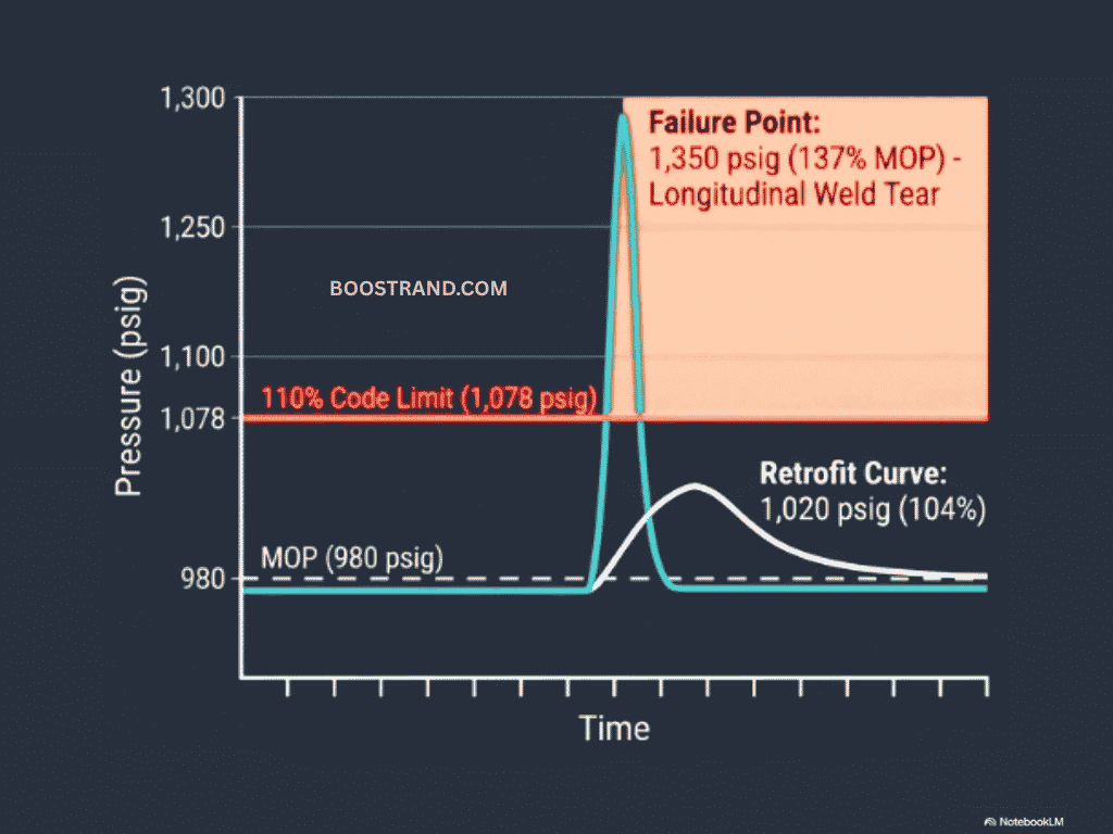
So when carrying out the surge analysis, we shall need to compare the maximum pressure at surge wave with these limits. If the required operating or transient conditions cannot be satisfied within that limit, surge protection measures shall be needed. These can either be:

1. Reduce the shutdown valve closure time and hence reduce the maximum surge pressure to ASME applicable limits.
2. Add Surge relief valves as a mitigation method to relieve excess pressure.

NOTE: ASME B31.3 and B31.4 represent the minimum requirements for maximum surge pressure. Always verify the applicable project criteria, as local or project-specific standards may impose more stringent limits.

So how shall we determine the protection requirements for a surge scenario? Let’s see.

---

Step 1 — Quantifying the Surge

In order to assess whether water hammer would be an applicable overpressure scenario or not, we shall need to quantify the surge scenario. This can be done by 2 methods:

1. The Joukowsky Equation: Which is a fast and preliminary rule of thumb. However, it’s results won’t be accurate. It can just be a first-pass screening tool only. If the Joukowsky screening calculation shows the surge pressure is close to or above the ASME B31.4 allowable, then a dynamic simulation would be needed for more accurate results.
2. Detailed Surge Analysis: Through a rigorous software such as Synergi Pipeline Simulator (SPS), Pipe Studio, AFT Impulse, Bentley HAMMER, PIPENET Transient, or HYSYS Dynamics. This analysis would be needed to quantify the surge wave, maximum flow through surge relief valve, and expected surge volume to downstream surge relief system sizing. This analysis can also determine the required valve closure time that can eliminate overpressure.

The Joukowsky Equation

The Joukowsky equation is the starting point for any surge awareness exercise. It assumes ideal conditions that never exist in real pipelines: a single uniform pipe segment, perfectly incompressible fluid, instantaneous and complete flow stoppage, and no wave reflections, friction, or system boundary effects. The instantaneous surge pressure rise following a sudden flow stoppage is:

$$\Delta P = \rho \cdot a \cdot \Delta V$$Where:

• ΔP = instantaneous pressure rise (Pa)
• $\rho$ = liquid density (kg/m³)
• $a$ = pressure wave speed (m/s)
• ΔV = change in fluid velocity (m/s)

The pressure wave speed $a$ is calculated as:

$$a = \sqrt{\dfrac{K/\rho}{1 + \dfrac{K \cdot D}{E \cdot e}}}$$Where:

• $K$ = fluid bulk modulus (Pa) — for water: 2.2 × 10⁹ Pa; for crude oil: ~1.5 × 10⁹ Pa
• $\rho$ = fluid density (kg/m³)
• $D$ = pipe internal diameter (m)
• $E$ = pipe Young’s modulus (Pa) — for carbon steel: ~207 × 10⁹ Pa
• $e$ = pipe wall thickness (m)

Surge wave speed varies significantly with fluid and pipe material — ranging from 1,400–1,500 m/s for water in a rigid pipe down to 100–300 m/s for liquid with entrained free gas — governed primarily by fluid bulk modulus, pipe wall stiffness, and fluid density.

For water ($\rho$≈1,000 kg/m³) in steel pipe with a wave speed of $a$≈1000 m/s, a sudden velocity change of $\Delta V = 1$m/s gives ΔP=10 bar. In dense liquid hydrocarbon lines, the pressure rise per unit velocity change is higher because density is greater.

Why the Joukowsky Equation Is Never Enough: The Case for Dynamic Simulation

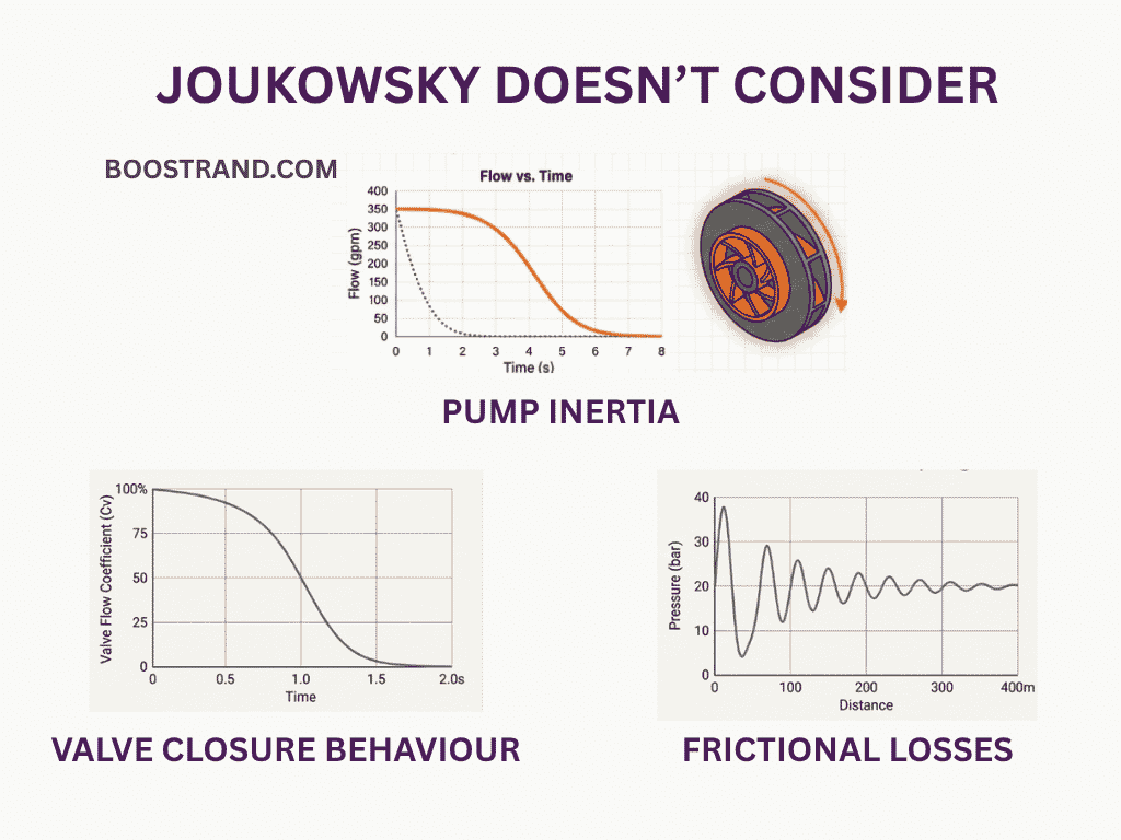
The Joukowsky equation has no knowledge of the following — all of which affect the real surge pressure in a pipeline system:

• Pump inertia and trip curve: After a pump trips, it does not stop instantaneously. The rotating assembly decelerates over seconds, modifying the pressure-time profile at the pump discharge significantly
• Check valve dynamics: A non-slam check valve closes over a finite time that interacts with the decelerating flow; the slam spike depends on the reverse velocity at closure, not just the initial forward velocity
• Pipe friction: Friction attenuates the wave as it travels; Joukowsky ignores this entirely
• Wave reflections from system boundaries: Every change in pipe diameter, branch, dead-end, and open tank reflects waves that interact with the primary wave
• Line pack: In long pipelines, when a downstream valve closes or ESD activates, the upstream pumps continue running for the wave travel time $(2L/a)$ before pump trip logic activates. During this window, pumps continue adding energy to the trapped fluid column — generating pressures significantly higher than Joukowsky alone predicts.
• Multiple pumps, parallel branches, and complex network topology: All interact simultaneously during a transient, which need a rigorous software to correctly predict the surge behavior.

Line pack deserves particular emphasis in long-distance pipeline design. As pipeline length increases, the pipe period $(2L/a)$ increases proportionally. Let’s see the below scenario:

• For a 50 km crude oil pipeline with a wave speed of 1,100 m/s, the pipe period is about 91 seconds.
• During those 15 seconds, pumps continue adding energy to the trapped fluid, causing pressures much higher than predicted by a simple Joukowsky pump-trip calculation.
• If the ESD trip logic needs 10–15 seconds to detect downstream valve closure and send the trip signal, upstream pumps keep running during that interval.
• Therefore, automatic pump trip interlocks must act within the time window set by the pipe period to prevent excessive surge pressures.

The only tool that captures all of these effects simultaneously is a rigorous, calibrated dynamic transient hydraulic simulation — run in purpose-built software with real equipment boundary conditions, real pipe geometry, and real operating scenarios.

These tools model complex boundary conditions including pumps with inertia and trip curves, valves with actual Cv-versus-position characteristics and actuator timing, surge relief valves with opening and closing time constants, accumulators, column separation, wave reflections, and pipe network topology simultaneously. The Joukowsky equation models none of this.

When to Perform Surge Analysis in the Project Lifecycle

Surge analysis is not a one-time check performed at the end of design. It must be integrated into the engineering workflow at multiple stages:

Project Stage	Scope
Conceptual / FEED	Identify surge-sensitive segments; define protection philosophy; select preliminary surge protection device types. Avoids costly redesign during detailed engineering.
Detailed Design	Full transient hydraulic simulation of all pump trip, ESD, and valve closure scenarios. Verify pipe stress inputs for support design. Size all surge protection devices and confirm valve closure time requirements.
Operational Changes and Debottlenecking	Any modification that changes flow rate, pipeline length, pump configuration, or valve arrangement requires reassessment of surge behaviour. The surge model built during design is a reusable engineering asset.

Initiating surge analysis during FEED, not at the end of detailed design, is the single most cost-effective decision in surge protection engineering. Retrofitting surge protection hardware into a completed design is significantly more expensive than incorporating it early.

---

Step 2 — Choosing Surge Protection Measures

So let’s assume that based on the surge analysis that was made, the maximum surge pressure was found to be higher than the pipeline design pressure by more than 10% allowed by ASME 31.4. Here we have 3 options:

1. Preventing the surge wave from reaching extremely high pressure: This can be done by increasing valve closure time or adding other considering variable speed drive or some shutdown sequence for upstream pumps.
2. Designing the pipeline to withstand maximum surge pressure: if the valve closure time cannot be further reduced or won’t help a lot.
3. Adding Surge Relief Valves (SRV): to relieve the excess pressure to an open system.

Valve Closure Time Extension

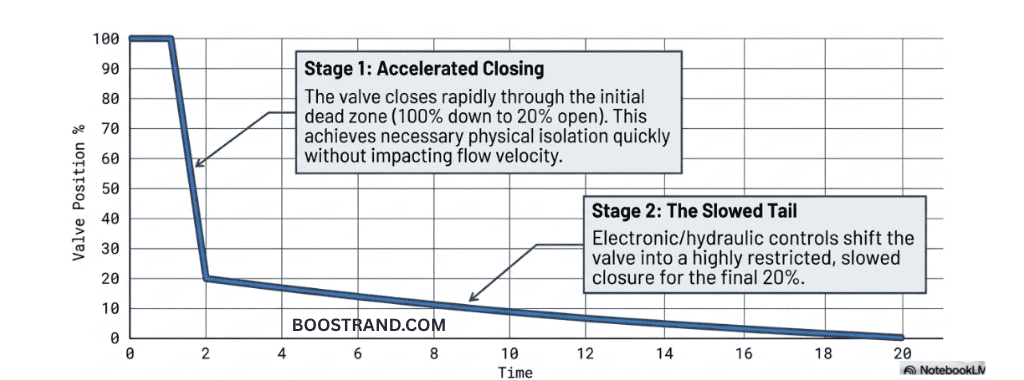
Extending ESD/MOV valve closure time is the most cost-effective prevention measure. The rule of thumb is 1 second per inch of valve size (e.g., a 10-inch ESD valve: minimum 10 seconds to close). For valves larger than 12 inches (300 mm), a minimum of 15 seconds is commonly applied, with the dynamic simulation potentially requiring 30–120 seconds depending on pipeline length and allowable pressure margin.

Different valve types have different effective closure phases — the critical interval during which flow actually reduces. The below table shows an example of closure phases (figures are just for illustration but need to be confirmed during a project):

Valve Type	Effective Closure Phase (flow-reducing travel)
Gate valve	Last 5% of travel
Butterfly valve	Last 15% of travel
Ball valve	Last 25% of travel
Plug valve	Last 30% of travel

A two-speed actuator (fast for the first 75–85% of travel, slow for the final critical phase) provides an effective compromise between emergency shutdown speed and surge pressure control.

---

Step 3 — Design of Surge Relief System

So if the valve closure time won’t fulfill ASME requirements for surge and pipeline design pressure couldn’t be increased, the only solution would be to mitigate the surge scenario through surge relief valves.

Surge Relief Valves (SRVs) are the primary active protection device in liquid pipeline surge relief systems. Under normal operating conditions, the valve remains closed. When a surge event causes pipeline pressure to exceed the valve set point, the SRV opens automatically and immediately — discharging sufficient liquid through a relief line to a surge relief tank to prevent the pressure from exceeding the allowable limit. As the surge dissipates, the valve closes in a controlled manner and remains ready for the next event.

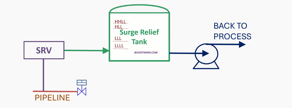
So here, adding SRV is not just about a relief valve. It’s a full surge relief system. This comprises of:

1. Surge Relief Valves (SRV)
2. Relief Piping from SRV to the downstream tank/vessel
3. Tank or vessel to receive the relieved fluid
4. Pump and piping to return the relief fluid from the relief tank back to upstream operation or to another facility. Here, the relieved fluid can be reused. In addition, the tank will be kept empty so that it won’t overfill in case the SRV opened again.

How is SRV different from a typical PSV

Surge scenario is more dangerous than a typical overpressure scenario as it’s highly instantaneous. That’s why a typical PSV designed as per API 520 won’t fit as a protection against water hammer and a different relief device would be needed.

The fundamental performance requirements for a pipeline SRV are:

• Fast acting — must reach full open capacity in under 100 milliseconds in high-severity applications
• High capacity — must be capable of passing the full surge relief flow rate
• Controlled closure — must re-close slowly and in a controlled manner to avoid generating a secondary surge; closing times of 20 to 60 seconds are typical for liquid pipeline applications

Types of Surge Relief Valves

1. Gas-Loaded (Nitrogen-Loaded) Surge Relief Valves

Balanced Piston Design:

• Normally closed; opens on increasing inlet pressure exceeding the nitrogen pre-charge
• The gas pressure set point, minus the valve spring force (typically ~0.28 barg / 4 psi), is the effective surge relief set point
• Response time typically under 100 milliseconds
• An integral oil reservoir on the cylinder head provides unrestricted flow when opening and a reduced orifice to limit closing speed — preventing secondary surge from rapid valve closure

Design consideration for nitrogen system:

When the SRV opens, nitrogen volume decreases and consequently pressure increases within the gas plenum in the SRV. That’s why a buffer tank is needed to receive Nitrogen and keep the plenum pressure at a pressure close to the SRV set point. The nitrogen gas buffer tank must be insulated or buried underground to minimize temperature-driven pressure changes, which would shift the effective set point of the relief valve.

Surge Relief Valve Skid Configuration

In industrial practice, SRVs are supplied as factory-tested, skid-mounted packages:

• Redundant parallel SRVs — typically two or more in parallel for full capacity and maintenance isolation
• Full-port ball valves upstream and downstream of each SRV — provides lowest resistance path in the relief line
• Inlet and outlet manifolds sized to minimise pressure loss through the relief circuit
• Nitrogen supply and control system — pressure regulator, gauge, nitrogen bottles, insulated nitrogen buffer vessel, and electronic control system for set-point accuracy and monitoring
• Ultrasonic flow meter at the outlet of each SRV — monitors discharge volume during each valve cycling event for performance verification and post-event analysis
• Control panel and instrumentation — local pressure indication, high-pressure alarm, valve position indication

2. Pilot-Operated Surge Relief Valves

• Can control pressures to within ±2 psi (±0.14 bar) of set pressure, regardless of upstream conditions
• Relatively slower response time compared to gas-loaded designs
• Recommended only for clean, low-viscosity fluid applications

Surge Relief Valve Design Criteria

Design Parameter	Description	Reference
Set Pressure	Must be below or at the design pressure to leave room for the 10% surge allowance. The specific set point is the primary output of the surge transient simulation.	ASME B31.4 / Surge Analysis
Relief Flow Rate (Based on rated Cv)	The required discharge flow rate (m³/h or gpm) to limit surge pressure to the allowable level — determined from the transient simulation. The valve Cv must handle this flow with the available differential pressure.	Transient Simulation
Response Time	Time from set pressure exceeded to full valve opening. Typically < 100–200 ms. Gas-loaded designs typically achieve sub-100 ms. Required response time confirmed by transient simulation.	Industry practice
Valve Closing Time	Must be slow enough to avoid generating a secondary surge during closure. Typical range: 20–60 seconds for liquid pipeline applications. Achieved via oil dashpot or controlled orifice in the cylinder head.	Industry practice
Pressure Rise to Open	The additional pressure rise above the set point required to achieve full Cv — must be factored into the transient simulation model.	Industry practice

---

Surge Relief Tanks

When an SRV opens, the discharged liquid volume must be safely received. In hydrocarbon pipeline systems, this receiver is the Surge Relief Tank (also called a Surge Relief Drum or Surge Receiving Vessel).

Purpose of the Surge Relief Tank

The surge relief tank performs three functions:

1. Safely receives and contains the liquid volume relieved from the pipeline during a surge event — preventing environmental release of hydrocarbons
2. Provides volume buffer — absorbs the surge energy and allows pipeline pressure to return to acceptable levels
3. Stores product for re-injection — collected liquid is returned to the pipeline via a dedicated surge relief return pump after the event

Surge Relief Tank Sizing

Surge relief tank should be sized to ensure that it shall safely handle all surge volume without being overfilled. This means that the capacity of the tank from low liquid level to high liquid level should accommodate the relief capacity. This is also considering that the tank shall be emptied once the relief is finished.

But how do we determine the relief capacity?

The conservative approach is to multiply the maximum surge rate by the relieving time to get the relief volume. This shall yield the largest tank volume.

However, when looking at the simulation output, we find that the surge relief flow rate shall vary from the start of relief up to the end of relief as shown in the below curve.

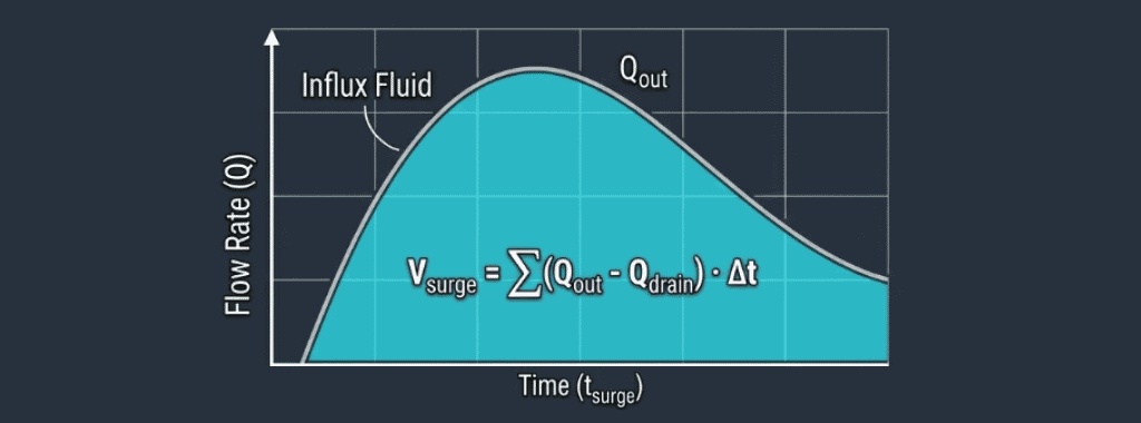
So here we can see that the minimum required tank volume is determined by integrating the SRV discharge flow rate $Q(t)$ over the full duration of the relief event from the transient simulation output. This can yield a tank with smaller dimensions and a more economic design.

$$V_{tank,\,min} = \int_0^{t_{event}} Q(t)\, dt$$

It’s highly important to mention here that the required tank volume should consider handling all credible worst-case scenarios (pump trip, ESD closure, power failure, accidental valve closure) so that the tank level does not exceed High-High Level and the pipeline pressure remains within the ASME B31.4 allowable limits.

Operating Levels

Surge relief tank size, same as any other tank, shall depend on the required capacity and how this capacity shall determine tank diameter and levels. The below table shows the basic criteria needed for tank sizing. You can also check out our Calcpad sizing tool for tanks to try out preliminary sizing for your storage tank.

Level	Criterion
Low Low Liquid Level (LLLL)	Minimum level at which the return pump shall be tripped to avoid cavitation and at which filling nozzle is submerged to avoid static electricity during filling.
Low-Liquid Level (LLL)	Level which represents the bottom of tank net capacity. This also represents the level at which there is an alarm to the operator to stop the return pump before tripping it through ESD.
High Level (HL)	Level which represents the top of tank net capacity (equivalent to HLL-LLL). Alarm setpoint — triggers early warning to control room
High-High Level (HHL)	Interlock to initiate additional response; set below maximum liquid level to prevent overflow
Maximum Liquid Level	Sized to leave minimum 10–15% gas space above liquid under worst-case fill condition

Tank Maximum Pressure And Static Head

The tank design pressure must accommodate the maximum vapor pressure of the fluid it is expected to accommodate as explained in the article Understand the Basis to Select Proper Storage Tank Type.

On the other hand, the maximum expected level at surge relief tank should be considered in the back pressure on SRV when carrying out the surge analysis as if can affect the SRV’s effective flow capacity (Cv) — high back-pressure reduces the pressure differential across the SRV, limiting its relief capacity. This interaction must be modelled in the transient simulation.

Inlet Nozzle Design

The inlet nozzle sizing is governed by two separate criteria:

Erosion velocity

This is the typical pipe sizing criterion as explained in the article Pipe Sizing Criteria and Calculation Procedure for Process Engineers. This ranges from 3 – 6 m/s depending on the pipe material.

Electrostatic ignition limit (API RP 2003 — governing for hydrocarbon service):
The inlet nozzle must be sized based on the maximum SRV discharge flow rate at a velocity ≤ 1 m/s per API RP 2003. This is a fire and explosion hazard — not a mechanical concern. In hydrocarbon service, this criterion is more restrictive than any erosion velocity limit. API RP 2003 states it as follows:

1. Filling velocity of the incoming liquid stream to 1 m/s (3 ft/s) until the fill pipe is submerged either two pipe diameters or 61 cm (2 ft), whichever is less.
2. For static accumulator liquids (refined petroleum products with electrical conductivity below (~50 pS/m) with any dispersed water phase present, this limit applies throughout the entire filling operation.

So here we see that electrostatic ignition limit can be the more stringent criterion if the liquid is a static accumulator or if liquid cannot be submerged enough. For surge relief where the initial surge flow is the maximum flow, surge relief tank level should be enough above the required submergence level if the velocity criterion cannot be achieved.

This can also be achieved by adding an inlet device such as a submerged dip pipe (extended below the Normal Operating Level) combined with an internal splash baffle or distributor — to ensure the liquid enters below the liquid surface as quickly as possible and minimizes the duration of above-liquid-level filling.

---

Surge Relief Return Pumps: Closing the Loop

Without a return pump, the surge relief tank fills after successive surge events and eventually loses its available protective volume. The Surge Relief Return Pump (pump-back pump) returns the collected liquid from the tank to the pipeline or upstream source vessel.

The return pump does not participate in the surge protection event itself — that event occurs in milliseconds, while the pump-back cycle may take minutes to hours. The pump starts after the event, drains the tank to Normal Operating Level, and stops.

Pump rated flow should consider a high flow enough to empty the tank within a small amount of time (typically 30–60 minutes) so that tank would be ready as soon as possible for any new surge wave. Other pump sizing parameters shall follow typical pump sizing parameters. You can check out our Pump Hydraulics & Sizing Course to understand these parameters more and also Calcpad pump sizing tool for preliminary pump sizing.

---

Pipe Supports and Structural Coordination

A surge relief design is not complete until its implications for pipe structural loading have been addressed. This is a coordination point frequently missed in projects where surge analysis and pipe stress engineering run as separate, unconnected workstreams.

During a surge event, the transient pressure wave exerts net hydraulic force on every change in pipe geometry — bends, reducers, branch tees, and closed ends. These transient forces are dynamic, directional, and can significantly exceed the steady-state pressure thrust loads that are used as the basis for support and anchor design in conventional pipe stress analysis. That’s why surge scenario should be well studied by the piping stress engineer.

---

Worked Calculation Example

This example demonstrates first-pass Joukowsky screening only. The numbers produced here must be followed by a full dynamic simulation before any design decisions are made.

GIVEN:

• Pipe: NPS 20, OD 508 mm, wall thickness $e$e = 9.53 mm → ID = 488.9 mm
• Fluid: Crude oil, $\rho$ = 850 kg/m³, bulk modulus $K$ = 1.5 GPa
• Pipe material: Carbon steel, $E$ = 207 GPa
• Segment length to nearest source: $L$ = 20 km
• Normal flow velocity: $V_1$​ = 1.8 m/s
• Event: Pump trip with fast check valve closure → $V_2$= 0 m/s
• MOP = 90 barg; operating pressure at point of interest = 75 barg

FIND: Wave speed $(a)$(a), Joukowsky pressure rise $(\Delta P)$(ΔP), critical closure time $(T_p)$(Tp​), and ASME B31.4 compliance check.

SOLUTION — Wave Speed:

$$\frac{K}{\rho} = \frac{1.5 \times 10^9}{850} = 1{,}764{,}706 \text{ m}^2/\text{s}^2$$$$\frac{K \cdot D}{E \cdot e} = \frac{1.5 \times 10^9 \times 0.4889}{207 \times 10^9 \times 0.00953} = 0.372$$$$a = \sqrt{\frac{1{,}764{,}706}{1 + 0.372}} = \sqrt{1{,}285{,}500} \approx 1{,}134 \text{ m/s}$$Sanity check: Rigid pipe upper bound = $\sqrt{K/\rho} = \sqrt{1{,}764{,}706} \approx 1{,}329$ m/s.

Calculated value of 1,134 m/s is below this — confirmed reasonable.

SOLUTION — Joukowsky Pressure Rise:

$$\Delta P = 850 \times 1{,}134 \times 1.8 = 1{,}732{,}000 \text{ Pa} \approx 17.3 \text{ bar}$$Peak transient pressure = 75 + 17.3 = 92.3 barg

ASME B31.4 ceiling = 1.10 × 90 barg (MOP) = 99.0 barg

→ 92.3 barg < 99.0 barg — within the ASME B31.4 surge limit at this operating condition, with 6.7 bar (97 psi) of margin.

SOLUTION — Critical Closure Time $(2L/a)$ :

$$T_p = \frac{2 \times 20{,}000}{1{,}134} \approx 35 \text{ seconds}$$→ Any valve closing in less than 35 seconds at this location must be treated as instantaneous and designed for the full 17.3 bar rise.

What if operating pressure is higher? Run the same case with operating pressure at 85 barg (a busier flow period, closer to MOP):

Peak transient pressure = 85 + 17.3 = 102.3 barg — now 3.3 bar above the 99.0 barg B31.4 ceiling.

If the higher pressure in the pipeline is related to higher friction losses due to higher flow, this would mean that normal fluid velocity is higher, which shall need to be considered in the equation and would even lead to a higher pressure. This would also apply in case the pipeline was serving a fluid with a higher density or bulk modulus leading to a higher pressure rise.

Surge relief is no longer optional. This is exactly why a surge study must evaluate a range of operating conditions, not only the nominal case — and why the Joukowsky result showing a B31.4 breach must immediately trigger a full dynamic simulation to ensure the surge is accurately quantified.

---

Summary of Key Design Criteria

Component	Key Design Criterion	Reference
Allowable surge overpressure — liquid pipeline	Max 10% above internal design pressure	ASME B31.4 para. 403.3.4
Allowable surge overpressure — process piping	Max 33% above design pressure (time-limited; ≤ 10 hrs/event; ≤ 100 hrs/year)	ASME B31.3
Surge analysis method	Full dynamic simulation required (SPS, Pipe Studio, AFT Impulse, PIPENET, etc.); Joukowsky for first-pass screening only	ASME B31.4 / Industry practice
SRV response time	< 100 ms (gas-loaded); confirmed by transient simulation	Industry practice
SRV closing time	20–60 seconds — must not generate secondary surge	Industry practice
Tank volume sizing	Determined by integrating SRV discharge flow Q(t) over event duration from transient simulation	Industry practice
Gas-charged vessel sizing	Polytropic basis: $P_0 V_0^n = P_{max} V_{max}^n$​; $n$ = 1.2–1.4 for nitrogen; min. 20% liquid buffer above outlet nozzle	ASME Section VIII / Industry practice
Tank inlet velocity	≤ 1 m/s (3 ft/s) to prevent electrostatic ignition in hydrocarbon vapor space	API RP 2003 §4.5
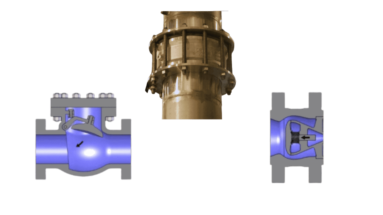
Pump discharge check valve	Non-slam (nozzle/spring type) Check out Swing vs non-slam check valve	Industry practice
ESD valve closure time	≥ 1 sec per inch of valve size; Can be increased based on surge analysis requirement to prevent overpressure	Industry practice
Pipe support coordination	Transient force data must be extracted from the simulation and issued to pipe stress engineering	Industry practice

Share this:

[…] creation of a PFD is typically based on the output of process simulation software. We have discussed plant simulation’s role in a project in the previous article. In a nutshell, process simulation involves using specialized software to model and analyze the […]